Understand the incident investigation workflow
The starting problem was the effort involved in investigating recurring IT operations incidents. Historical tickets and their resolution notes can contain useful experience, but the existing approach needed manual labels to train its models. A separate stream of metric data could help identify when a system was behaving unusually. The project explored how these two streams could support an operator’s investigation.
I began by running the existing code, reviewing the model logic and documenting the current approach. The internship report places this work in the SmartOps context, with broader interests in monitoring, predictive analytics and workflow automation. Those platform capabilities are background to the internship, rather than features implemented by this portfolio page.
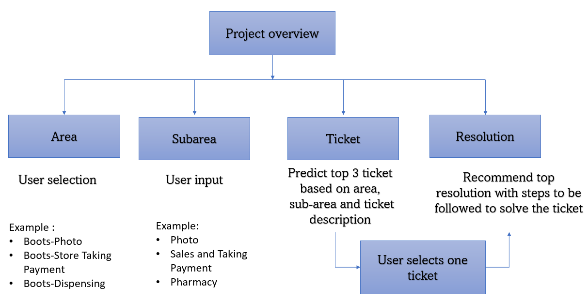
The ticket workflow starts with the user selecting an area and subarea, which narrow the problem domain. The system then presents related tickets; the user chooses the most relevant one, and associated resolutions are ordered by a quality score. The original flow diagram describes presenting the top three ticket candidates. A person remains responsible for selecting the relevant incident and assessing the proposed resolution.
The practical outputs were candidate ticket pairs, resolution-quality labels and scores, forecasts of expected metric behaviour, and anomaly flags. Together they provide evidence for investigation. Text similarity and unusual metric values do not, by themselves, prove a causal relationship or confirm a remedy.
and subcategory
historical tickets
for the chosen ticket
Recreated from the report’s Word drawing and adjacent workflow description. The operator selects the relevant ticket before reviewing resolutions.
 View full size ↗
Choose the area and subarea, review related tickets, select a ticket and inspect ranked resolutions.
Prepare the ticket and resolution data
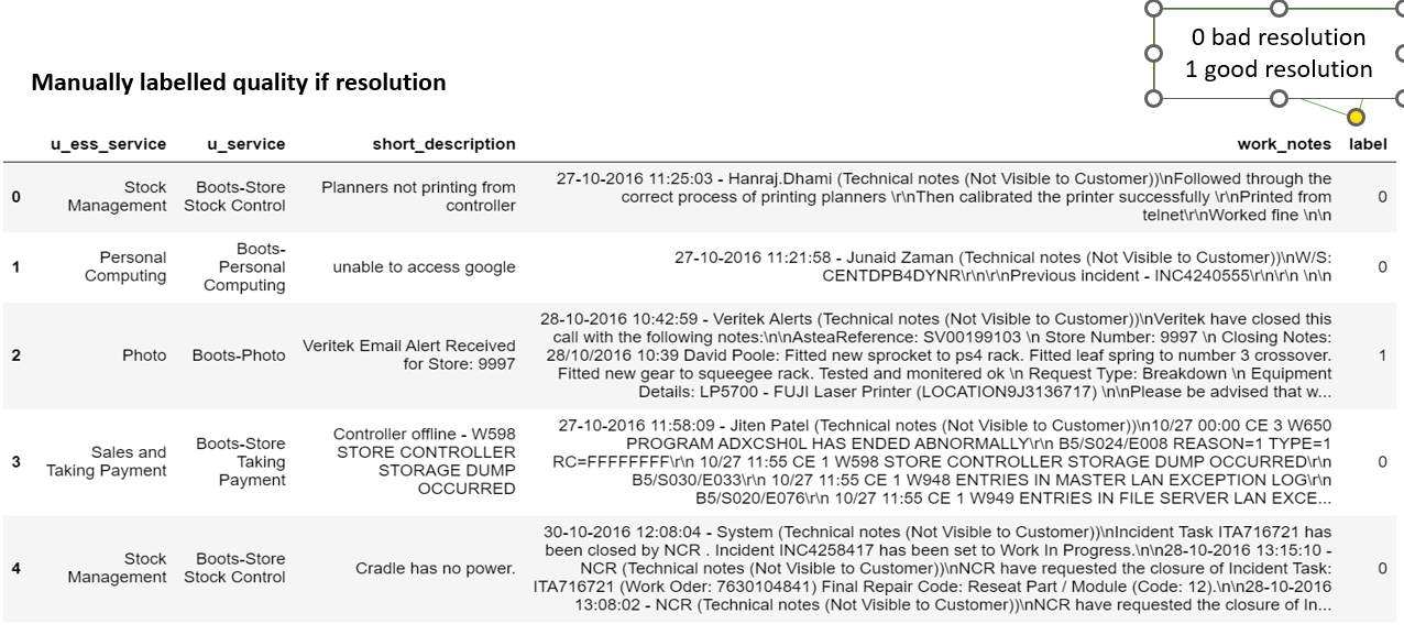
The recommendation data separates the problem domain from the description of the incident. In the report’s resolution dataset, u_service denotes the area and u_ess_service denotes the subarea. The illustrated records also include short descriptions, work notes and a manually assigned resolution-quality label. These fields serve different purposes: domain fields narrow the search, the description represents the problem, and work notes describe what was tried.
A key preparation issue was that area and subarea had been concatenated with the ticket text. Two unrelated incidents could therefore share the same domain words and appear artificially similar. I extracted the actual incident description before vectorising it for cosine similarity, retaining the domain information separately for the selection workflow.
For resolution scoring, the existing approach used structured and linguistic features derived from activity notes. The report lists action and problem counts, activity count, last-activity length, part-of-speech ratios, punctuation and number ratios, acronym counts and ratios, a length-range indicator, SLA status, and counts of knowledge-base references, IP addresses and server names. These features describe the contents and structure of the notes; they are not direct evidence that an incident was resolved correctly.
The report records 4,266 instances in the ticket-similarity evaluation, covering 248 subareas and 28 areas. The sentiment experiments report 3,038 resolution instances. These are separate evaluations and should not be treated as a single shared test set. The figure below preserves the dataset illustration from the report; the underlying ticket dataset and employer application are not included in this website.
 View full size ↗
Historical sample rows from the report, including area, subarea, description, work notes and manual quality labels.
Generate candidate ticket-similarity labels
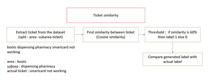
The original ticket model depended on manual similar/not-similar labels. To reduce that labelling effort, I explored a rule based on cosine similarity between vectorised incident descriptions. The sequence was: remove the area/subarea prefix, vectorise the remaining ticket text, compare ticket pairs, apply the similarity threshold, and compare the generated labels with the available reference labels.
Cosine similarity measures the alignment of two vectors: cosine(A, B) = (A · B) / (‖A‖ × ‖B‖). A higher value means the representations point in a more similar direction. In this experiment, the report uses a 60% similarity threshold to generate a positive label; pairs below the threshold receive a negative label. The precise vectoriser configuration and treatment of a score exactly at the boundary are not specified in the report.
These labels are algorithm-generated training signals, sometimes called weak labels. A pair can share vocabulary without sharing a cause, while two descriptions of the same issue can use different language. For that reason, the threshold should be understood as an experimental labelling rule, rather than a 60% probability that two incidents have the same cause.
The recorded evaluation compares these cosine-based labels with reference labels. Its 82% rounded accuracy belongs to this labelling experiment. It should not be presented as the end-to-end accuracy of the neural ticket recommender or as the accuracy of root-cause identification.
 View full size ↗
Extract the incident text, calculate cosine similarity, apply the 60% threshold and compare with reference labels.
Represent ticket pairs with a bidirectional LSTM
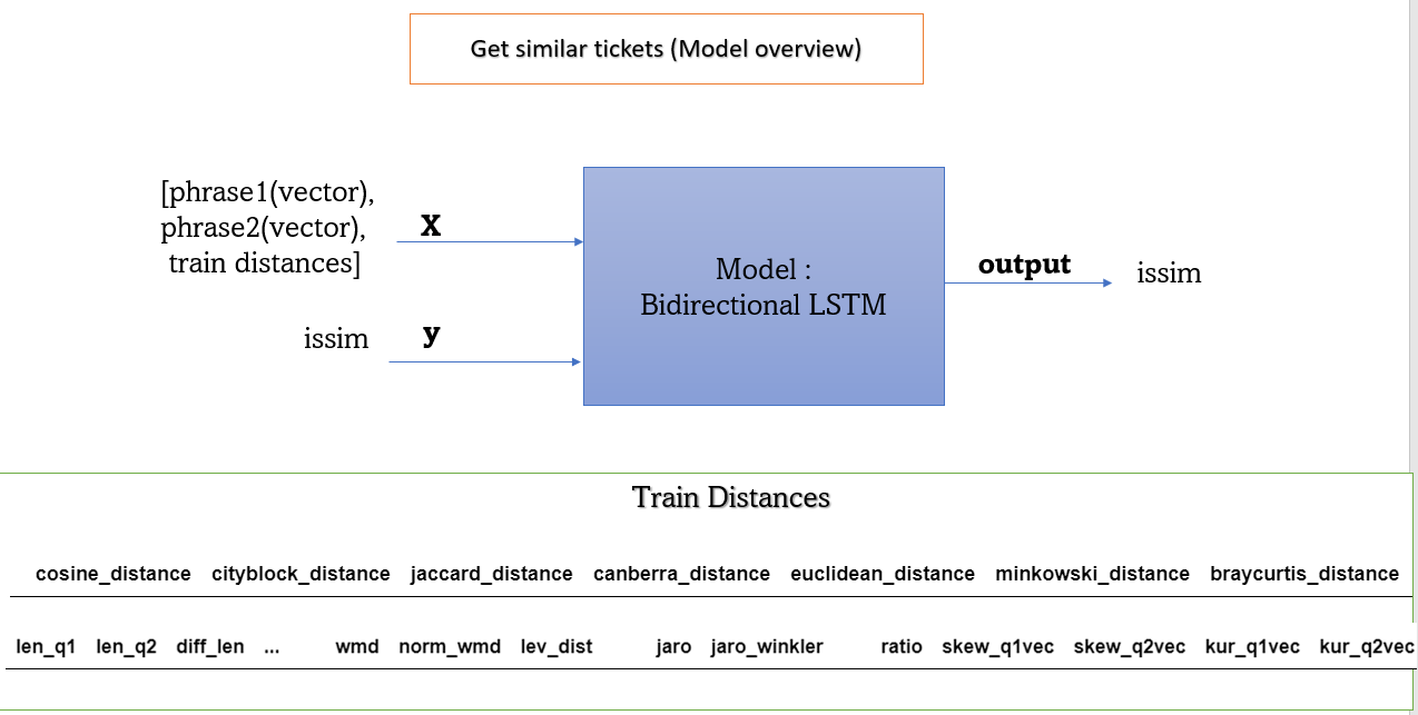
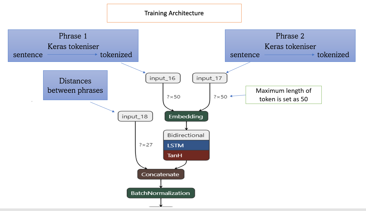
The existing similarity architecture takes three inputs: the first ticket, the second ticket, and a set of numerical distances and text-comparison features. Each ticket sentence is tokenised with the Keras tokenizer and passed through an embedding layer. The architecture figure specifies a maximum token length of 50.
The embedded ticket representations pass through a bidirectional LSTM. For text, the two directions allow the representation to use context from both earlier and later words within the supplied sentence. This use of a bidirectional model for ticket text is distinct from the chronological forecasting model used later for metric data.
The numerical branch describes relationships between the two tickets. The report discusses city-block and Canberra distances; ticket, word and character lengths; differences in length; common-word counts; word mover’s distance and its normalised form; and Levenshtein distance. The model overview also illustrates other distance and similarity measures. The exact feature-selection and preprocessing code is not supplied with the report.
The neural representation is concatenated with the comparison features, followed by batch normalisation and an output representing similar or not similar. The stated target uses 1 for similar tickets and 0 for non-similar tickets. This model supports candidate retrieval within the user’s chosen domain; the user then selects the ticket that best matches the actual problem.
The report documents this architecture as part of the existing workflow I studied and extended with automatic label generation. It does not provide a separate held-out performance table for the full bidirectional LSTM recommender, so the cosine-label evaluation is kept separate in the results section.
 View full size ↗
Two ticket representations and numerical comparison features enter the bidirectional LSTM similarity workflow.
 View full size ↗
Tokenisation, embeddings, bidirectional LSTM, concatenation with distance features and batch normalisation.
Experiment with labels for resolution quality
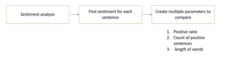
Resolution-quality training also required manual labels. I explored whether sentiment and simple text characteristics could generate candidate good/bad labels. The working assumption was that a useful resolution might finish with a positive statement or contain a higher proportion of positive sentences. This is a heuristic: positive wording alone does not establish technical correctness, completeness or a successful outcome.
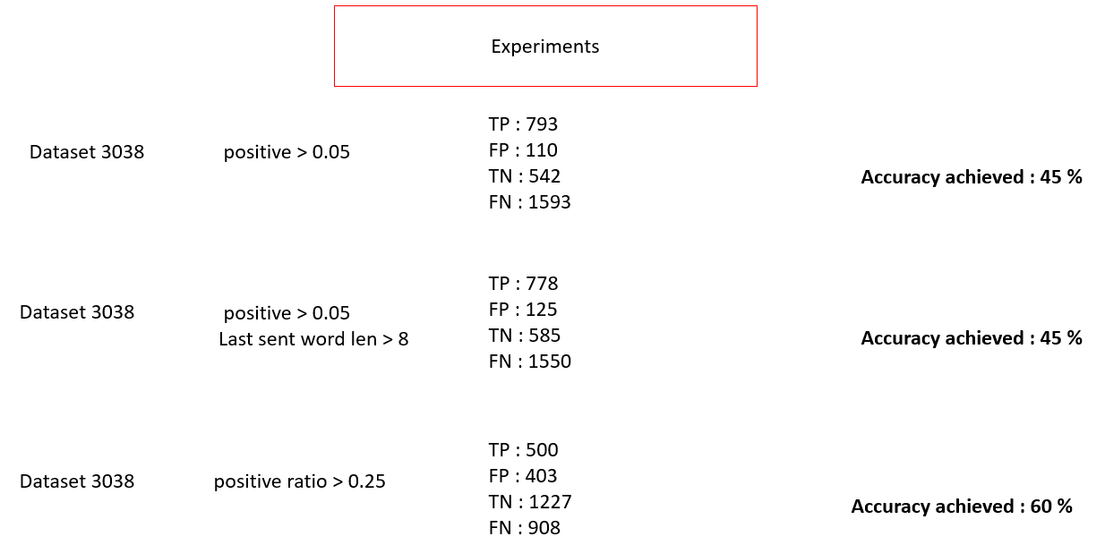
The workflow splits resolution text into sentences, obtains sentiment for each sentence, and compares alternative rules. The report shows three experiments: a sentiment score greater than 0.05; that score combined with a last-sentence word-length condition greater than 8; and a positive-sentence ratio greater than 0.25. The report does not fully specify the sentiment model or the precise meaning of the last-sentence length feature.
For the ratio approach, the idea is to divide the number of positive sentences by the total number of sentences in the resolution. This gives a summary of wording across the conversation, instead of relying on one score alone. The figure records a dataset size of 3,038 for each experiment.
The displayed accuracy labels are 45%, 45% and 60%. Recalculating accuracy from the printed confusion counts gives approximately 43.94%, 44.87% and 56.85%. The mismatch is retained transparently in the table below. The positive and negative reference totals also change between the experiments despite the same displayed dataset size; the report does not explain why. These results support a cautious comparison, not a definitive winning model.
The main lesson is that resolution quality is harder to infer than sentiment. Neutral, concise technical notes can describe a successful fix, and positive language can accompany an incomplete one. The report discusses comparing several parameters and finalising an approach, but does not supply enough implementation detail to reproduce a definitive selected label generator.
| Rule | TP | FP | TN | FN | Printed | Calculated |
|---|---|---|---|---|---|---|
| Sentiment > 0.05 | 793 | 110 | 542 | 1593 | 45% | 43.94% |
| Sentiment > 0.05 + length > 8 | 778 | 125 | 585 | 1550 | 45% | 44.87% |
| Positive-sentence ratio > 0.25 | 500 | 403 | 1227 | 908 | 60% | 56.85% |
Accuracy = (TP + TN) / (TP + FP + TN + FN). TP: true positives; FP: false positives; TN: true negatives; FN: false negatives. Figure 15 is preserved unchanged below.
 View full size ↗
Sentence sentiment, the positive-sentence ratio and text-length characteristics are explored as labelling signals.
 View full size ↗
Three rules evaluated on a stated 3,038 instances. Printed accuracy labels and confusion counts do not fully agree.
Use XGBoost to score and rank resolutions
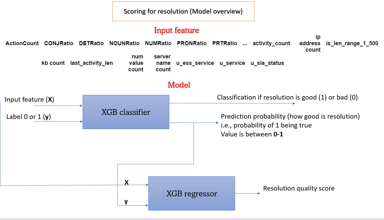
The documented scoring architecture first passes the engineered resolution features into an XGBoost classifier. Its target is the good/bad resolution label. Along with the binary classification, the classifier produces a probability-like output between 0 and 1 for the labelled positive class. Without calibration evidence, that number should not be interpreted as a verified chance that a proposed action will fix the incident.
The classifier output is then combined with the feature inputs for an XGBoost regressor, which produces a resolution-quality score. In the recommendation workflow, that score orders the candidate resolutions for the ticket the user selected. The result is a ranked set of historical suggestions for a person to inspect.
The sentiment work sits upstream of this architecture: it explores how training labels might be generated with less manual effort. Errors in those labels could affect both the classifier and the resulting ranking. The report’s sentiment accuracy figures therefore cannot stand in for a measured ranking-quality score.
The report illustrates the classifier-to-regressor design, but does not give the regressor’s target-construction details, hyperparameters, calibration results or a held-out ranking evaluation. No automatic remediation or operational success rate is claimed here.
 View full size ↗
An XGBoost classifier feeds its output and the engineered features to an XGBoost regressor for a ranking score.
Prepare time-series data for normal-behaviour forecasting
The second workstream explored metric forecasting and anomaly detection. The report describes finding open-source time-series data and generating expected patterns for experimentation. It does not identify the exact dataset, sampling frequency, metric units or train/test split, which limits independent reproduction of the numerical results.
The modelling goal was to forecast expected normal behaviour and compare it with observations. When anomalous peaks remained in training data, the forecasting model could learn to reproduce them. I therefore explored removing outliers using a z-score approach before training on the normal-behaviour series.
A z-score expresses a value’s distance from a reference mean in standard-deviation units: z = (x − μ) / σ. The report identifies this method but does not specify the outlier cutoff or the exact procedure for replacing removed observations. Those choices matter because removing points can change the time spacing and because legitimate workload peaks can resemble outliers.
The documented flow is metric data → outlier check → cleaned normal-behaviour data → forecasting model → comparison with actual observations. LSTM and Prophet appear as candidate forecasting methods in the workflow; the architecture and numerical forecasting results presented in the report are for LSTM.
For a reproducible follow-up, time order would need to be preserved, preprocessing fitted only on the training period, and genuine anomalies retained in the evaluation period. These are methodological follow-up requirements, not additional checks claimed to have been completed in the 2023 experiment.
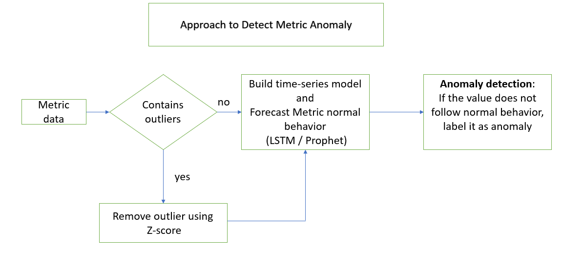 View full size ↗
Check for outliers, prepare normal-behaviour data, forecast the metric and compare actual values with expectations.
Add seasonality and calendar context
A single fixed expected value is a poor description of a metric with repeating workload cycles. The project explored hourly, daily and weekly seasonality, along with differences between weekdays and weekends and between office and non-office hours. The intent was to compare each observation with a relevant operating context.
The report describes four forecasting inputs: the metric value, a seasonal component, a weekday/weekend indicator and an office-hours/non-office-hours indicator. The seasonal component was obtained using seasonal_decompose from statsmodels; the calendar indicators were extracted from timestamps.
The next step was to construct input sequences and corresponding forecast targets. An input window gives the model a recent history; the output represents one or more future metric values. The supplied model code uses the variables n_steps_in, n_features and n_steps_out, but the report does not specify their final numerical settings or the decomposition period.
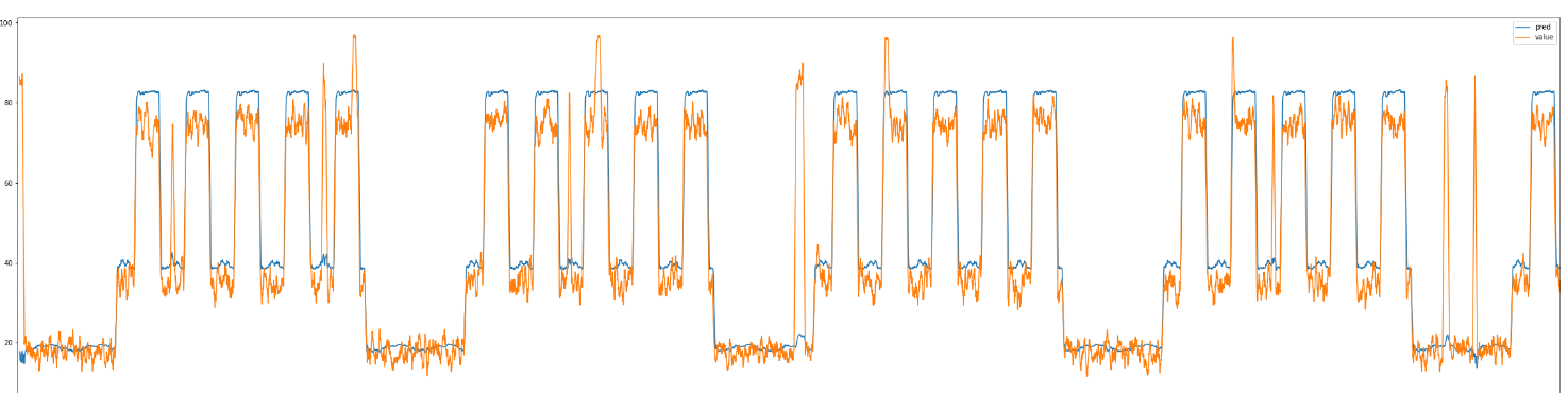
Both univariate and multivariate LSTM work appear in the internship task plan. The multivariate description adds seasonal and calendar information to the metric sequence. The accompanying forecast plot illustrates the model following repeated high- and low-activity periods. It is an experiment figure, rather than evidence of general performance across other systems.
The report uses an office-hours CPU-utilisation example to explain why contextual thresholds are useful. Those illustrative ranges are not measured project results. In a future reproduction, seasonal features must also be constructed without using observations from beyond the forecast cutoff.
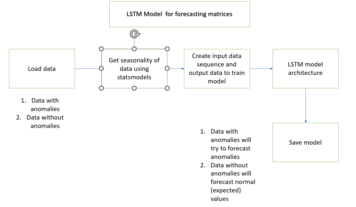 View full size ↗
Load the data, extract seasonality, construct input/output sequences, train and save the forecasting model.
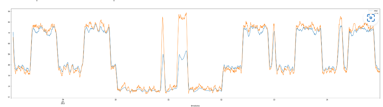 View full size ↗
The plotted forecast follows repeated activity patterns; the report describes value, seasonality, weekday and office-hours inputs.
Train the LSTM forecasting model
The supplied code builds a Sequential model with two LSTM layers of 100 units each. The first returns sequences so that the second can process the sequence output. A dropout layer with rate 0.2 follows the LSTM stack, and a dense layer produces n_steps_out forecast values.
The model is compiled with the Adam optimiser at a learning rate of 0.001 and mean squared error as the training loss. Training is configured for up to 100 epochs, with early stopping monitoring validation loss in min mode and patience set to 50. These are the settings visible in the report’s code figure; the figure does not show batch size or a random seed.
The code trains on trainX and trainy and passes testX and testy as validation_data. This means that the data called “test” participates in training decisions through early stopping. The report does not identify a further untouched holdout, so its error metric should not be described as a confirmed independent test score.
The forecasting pipeline also includes saving the trained model. The intended output is an expected normal metric trajectory against which actual observations can be compared. The original trained weights, training code and input datasets were not supplied with this report, so this portfolio page explains the experiment and displays its recorded figures rather than running that model.
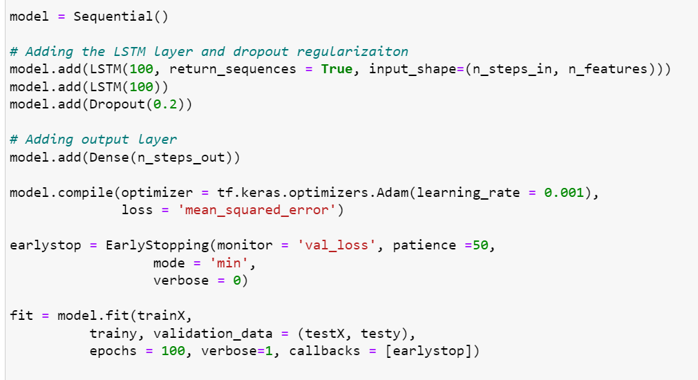 View full size ↗
The report’s code shows two 100-unit LSTM layers, dropout 0.2, Adam at 0.001, MSE and early stopping.
Compare two approaches to dynamic anomaly thresholds
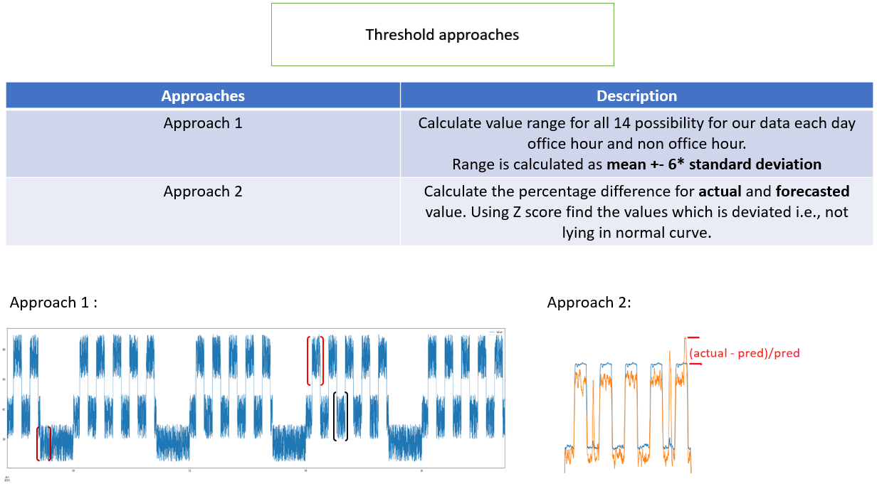
After forecasting, I explored two ways to turn deviations into anomaly flags. The first groups forecasted normal values by operating cycle. The report’s diagram describes 14 possibilities: each day of the week combined with office or non-office hours. For each group, the mean and standard deviation describe a context-specific expected range.
The first approach uses a range expressed in the figure as mean ± 6 × standard deviation. An actual observation outside the relevant group’s band is a candidate anomaly. This allows, for example, a Monday office-hours observation to be compared with its own expected context instead of a weekend or overnight baseline. Sparse groups and changing workloads can make the estimates unstable, and a wide band can miss anomalies.
The second approach works with the difference between actual and forecast values. Calculate the residual e(t) = actual(t) − forecast(t), describe the usual residual distribution with its mean and standard deviation, and identify unusually large departures. The figure also mentions percentage difference; the report does not resolve whether the final implementation used raw or percentage residuals. A final numerical cutoff for this approach is not supplied.
The distinction is what the threshold models: the first describes normal forecast levels within each operating context, while the second describes normal forecast error. The report presents the residual approach as requiring one threshold instead of separate cycle-specific thresholds.
A dynamic threshold is still a decision rule, not proof of a root cause. Its usefulness depends on false alarms, missed anomalies and detection timing. The later score figures are not explicitly mapped to one of these two threshold methods, so they are presented as the reported anomaly evaluation without assigning an unsupported method label.
 View full size ↗
Compare context-specific normal-value bands with thresholds based on the difference between actual and predicted values.
Evaluate the ticket labels and metric forecasts
For cosine-based ticket labels, the report records 1,645 true positives, 398 false positives, 1,860 true negatives and 363 false negatives. These add to 4,266 evaluated instances. Accuracy is (TP + TN) / total = 82.16%, consistent with the rounded 82% displayed in the source figure. Precision, recall and F1 calculated from the same counts provide additional context below.
The ticket evaluation indicates useful agreement with the available reference labels, with both false matches and missed matches remaining. It does not isolate the performance of the bidirectional LSTM or show whether users selected the correct resolution. The split strategy and independent label-audit procedure are not specified in the report.
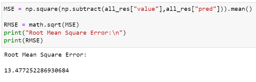
For metric forecasting, the report plots predicted and actual values and records a root mean squared error of approximately 13.47. RMSE = √mean((actual − predicted)²). It is measured in the units of the target series and penalises larger errors more heavily than smaller ones. It is not a percentage accuracy, and it is not the same as mean absolute error.
The screenshot shows 13.477252286930684; the report text shortens this to 13.47. The original value is preserved in the figure. Without metric units, a baseline model, a clearly separated holdout and the dataset itself, this error cannot establish performance across other workloads.
Forecasting the normal pattern also means that an unusual observed spike may intentionally differ from the forecast. The following step evaluates anomaly flags separately, because forecast error alone does not tell us how many incidents were detected or missed.
Calculated from the confusion counts in Figure 14. Precision, recall and F1 are additional calculations for this case study.
 View full size ↗
The 4,266 recorded instances produce 1,645 TP, 398 FP, 1,860 TN and 363 FN; accuracy rounds to 82%.
 View full size ↗
Original forecast plot from the report; the underlying series and metric units are not supplied.
 View full size ↗
The figure calculates RMSE and prints 13.477252286930684; the narrative reports approximately 13.47.
Evaluate anomaly detection and the smoothing tradeoff
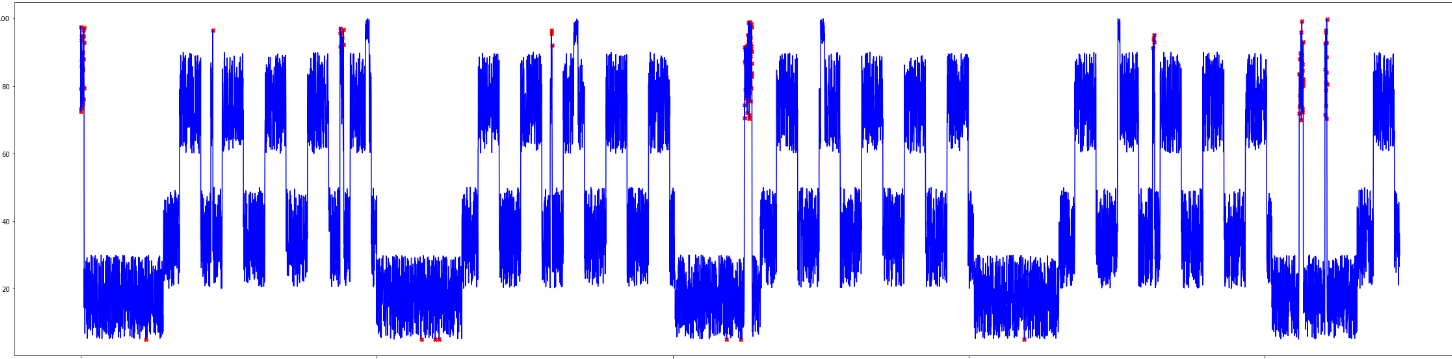
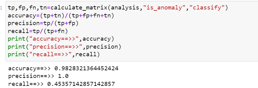
The report first evaluates anomaly decisions at individual time points. Figure 19 prints accuracy 0.9828321364452424, precision 1.0 and recall 0.45357142857142857. This corresponds to about 98.28% accuracy and 45.36% recall. The narrative elsewhere says 0.9889 accuracy; that is closer to the later averaged-result figure. This page uses the values printed in each figure and makes the discrepancy explicit.
Precision of 1.0 means no false-positive anomaly predictions in the recorded evaluation. It is not a guarantee that future alerts will always be correct. Recall of approximately 45.36% means that more than half of the labelled anomalies were missed. A high accuracy can coexist with poor anomaly coverage when normal observations dominate the data.
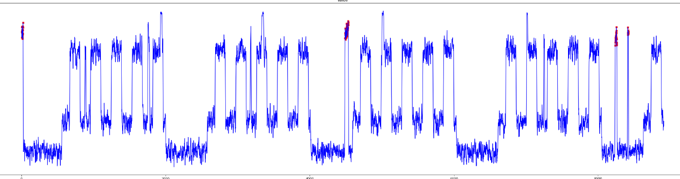
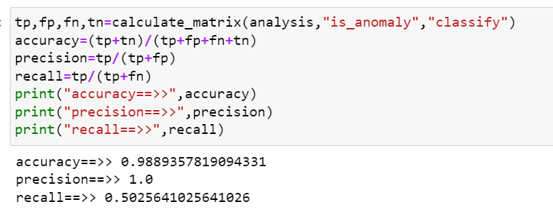
The report then averages over six data points and evaluates the smoothed result. Figure 21 prints accuracy 0.9889357819094331, precision 1.0 and recall 0.5025641025641026: approximately 98.89% accuracy and 50.26% recall. The figures show improved recorded recall, with about half the labelled anomalies still missed.
Smoothing can reduce isolated fluctuations, but it introduces detection delay and can blur short events. The report specifically notes lag from using the past six data points. Because the sampling interval is not stated, that lag cannot be converted into seconds or minutes.
The underlying labels, alignment rules and evaluation sample counts are not supplied for these two score figures. The comparison is therefore descriptive rather than a controlled proof of improvement. Event-level detection, detection delay, alert volume and performance on a separate chronological holdout would be useful next evaluations.
| Evaluation | Accuracy | Precision | Recall | Source |
|---|---|---|---|---|
| Individual points | 98.28% | 100% | 45.36% | Figure 19 |
| Six-point averaging | 98.89% | 100% | 50.26% | Figure 21 |
Rounded from the values in the screenshots. Evaluation counts and label alignment are not supplied; the comparison does not establish a controlled improvement.
 View full size ↗
Original plot of the metric series and pointwise anomaly indications.
 View full size ↗
Printed accuracy 98.28%, precision 100% and recall 45.36%, rounded here to two decimals.
 View full size ↗
The report explores averaging over six observations, with the tradeoff of detection lag.
 View full size ↗
Printed accuracy 98.89%, precision 100% and recall 50.26%, rounded here to two decimals.
Reflect on challenges and the next experiments
The first major challenge was representation: area and subarea words could dominate the actual incident description. Separating domain metadata from ticket text made the purpose of each input clearer. The wider lesson was that preprocessing decisions can change what a similarity model is really learning.
The second challenge was resolution quality. Sentiment and simple length rules were convenient ways to generate labels, but their recorded agreement was limited and the experiment figures contain inconsistencies. A stronger follow-up would use a consistent reviewed reference set and assess correctness, completeness and successful outcome directly, rather than treating tone as quality.
The third challenge was forecasting normal behaviour when training data included abnormal peaks. Exploring z-score outlier handling and calendar features helped frame the task around an expected baseline. It also highlighted the need to preserve time structure and evaluate the consequences of removing genuine workload variation.
The project strengthened my understanding of text representations, pairwise similarity features, bidirectional LSTM, feature engineering for XGBoost, time-series preparation, seasonal forecasting and the interpretation of precision and recall. It also reinforced the difference between an encouraging experiment and evidence sufficient to support a deployed system.
The report proposes future work on forecasting anomalies before they occur, adapting to changing seasonal patterns, correlating alerts across multiple metrics, and using ChatOps for notifications and guided investigation. It mentions STL, SARIMA, cross-correlation and multivariate models as possible directions. These are future ideas, not implemented features demonstrated here.
A research publication was planned at the time of the report. No publication record or completed production rollout is supplied in the source, so neither is claimed in this portfolio. The project remains a personal educational account of the internship work.
How the internship progressed
The detailed task plan records work from 12 April to 30 June 2023. The entries below retain the reported completion dates and distinguish delays where the plan gives them.
- 12–17 Apr 2023
Review and execute the existing code
Document the recommendation workflow and model inputs.
- 12–24 Apr 2023
Present the current approach and proposed changes
Identify manual-labelling dependencies.
- 24 Apr–12 May 2023
Explore cosine-based ticket labels
Planned finish 5 May; actual finish 12 May.
- 27 Apr–12 May 2023
Explore state and sentiment for resolution labels
Planned finish 5 May; actual finish 12 May.
- 12–15 May 2023
Update Python 3.10 compatibility
The task plan records compatibility work completed 15 May.
- 16–19 May 2023
Find open-source time-series data
Prepare the metric experiments.
- 18–28 May 2023
Research anomalies and multiple seasonal cycles
Study hourly, daily and weekly behaviour.
- 27 May–14 Jun 2023
Develop seasonal univariate LSTM
Planned finish 9 June; actual finish 14 June.
- 9–20 Jun 2023
Develop seasonal multivariate LSTM
Planned finish 15 June; actual finish 20 June.
- 12–20 Jun 2023
Explore mean and standard-deviation thresholds
Planned finish 19 June; actual finish 20 June.
- 20–30 Jun 2023
Work on anomaly forecasting
Task-plan entry; forecasting future anomalies remains a next-step topic in the conclusion.
Background reading listed in the report
These are the report’s references, reproduced as reading titles. Their presence does not validate the experiment results or imply that a publication was completed.
- Predicting Capacity Needs: How to Efficiently Monitor and Predict Capacity Needs with Capacity Analytics — Broadcom.
- An Anomaly Detection Algorithm for Microservice Architecture Based on Robust Principal Component Analysis — IEEE.
- AIOps Framework for Alerting Performance Issues in Microservices Using Time Series Forecasting — IJEAST.
- A Highly Efficient Modeling for Long Sequence Time Series Prediction in AIOps — arXiv:2211.07642.
- Time Series of Price Anomaly Detection with LSTM — Susan Li, Towards Data Science.
Personal educational portfolio. No employer endorsement, consulting service, commercial risk assessment or operational assurance is offered.